Pranav Rane
The Relic Abundance of WIMPs and Analysis of a Temperature Dependent Thermally Averaged Cross Section
Recent estimates suggest that over 26% of the universe is made up of matter that is undetectable by current methods. This strange, "dark" matter is important in the formation of galaxies and the structure of universe. One dark matter candidate is the weakly interacting massive particle (WIMP).
Introduction
The early universe was known to be hot and dense. Thus, particles in this stage of the universe did not have to travel far before interacting with other particles. This high probability for interaction generally kept the majority of particles in a state of equilibrium. For general chemical reactions taking the form
\[ a + b \rightarrow c + d \]
chemical equilibrium is maintianed such that
\[ \mu_{a} + \mu_{b} = \mu_{c} + \mu_{d} \]
However, if the rate of interactions was smaller than the rate of expansion then reactions could not occur rapidly enough for equilibrium to occur. This "out of equilibrium" phenomena resulted in abundances of certain particles, which play a key role in understanding:
- The formation of light elements in Big Bang Nucleosynthesis
- The recombination of protons and electrons into neutral hydrogen
- The possible production of dark matter
These three phenomena are a result of non-equilibirum physics. Further, these phenomena can be described by the Boltzmann equation for a reaction of the form \(1+2 \rightarrow 3+4\):
\[ \begin{gathered}a^{-3} \frac{d\left(n_1 a^3\right)}{d t}=\int \frac{d^3 p_1}{(2 \pi)^3 2 E_1} \int \frac{d^3 p_2}{(2 \pi)^3 2 E_2} \int \frac{d^3 p_3}{(2 \pi)^3 2 E_3} \int \frac{d^3 p_4}{(2 \pi)^3 2 E_4} \\ \times(2 \pi)^4 \delta^3\left(p_1+p_2-p_3-p_4\right) \delta\left(E_1+E_2-E_3-E_4\right)|M|^2 \\ \times\left(f_3 f_4\left[1 \pm f_1\right]\left[1 \pm f_2\right]-f_1 f_2\left[1 \pm f_3\right]\left[1 \pm f_4\right]\right)\end{gathered} \]
The Boltzmann equation is an integrodifferential equation for phase space distributions. The equation essentially states that the rate of change of the abundance of a particle is the difference between the rates of producing and eliminating the particle. If the righthand side is equal to 0, this means the magnitude of the number density of particle 1 times the scale factor cubed is conserved and does not change with time. Thus, the number density would be proportional to \(a^{-3}\).
The first line on the right hand side sums the overall momenta of the particles to find the total number of interactions. The second line on the right hand side represents momentum and energy conservation using continuous dirac delta functions where \( E=\sqrt{ p^{2}+(mc^{2})^{2} } \). The last line includes occupation numbers \(f\) that are functions of momentum, with a magnitude that depends on the species of the particles (1,2,3, or 4). Specifically, the value of an occupation number is dependent on the species of the particle as described by Bose-Einstein and Fermi-Dirac distributions:
\[ f_{BE} = \frac{1}{e^{(E-\mu)/T}-1} \tag{2.60} \] \[ f_{FD} = \frac{1}{e^{(E-\mu)/T}+1} \tag{2.61} \]
The Bose-Einstein distribution is used for bosons while the Fermi-Dirac distribution is used for fermions, where \( \mu \) is the chemical potential. However, our interest in the abundance of dark matter occurs when \( T << E-\mu \) which leads to \( f_{BE}\approx f_{FD} \). Thus, we can write the distributions as: \( f(E)\to e^{\mu/T}e^{-E/T} \).
Further, 3.3 can be used to rewrite the last line of 3.1 as: $$f_{3}f_{4}[1\pm f_{1}][1\pm f_{2}]-f_{1}f_{2}[1\pm f_{3}][1\pm f_{4}] \to e^{-(E_{1}+E_{2})/T}\left\{e^{(\mu_{3}+\mu_{4})/T}-e^{(\mu_{1}+\mu_{2})/T} \right\} \tag{3.4} $$ We can define the number density and equilibrium number density of particle \(i\) as: $$n_{i} = g_{i}e^{\mu_{i}/T}\int \frac{d^{3}p}{(2\pi)^{3}} e^{-E_{i}/T} \tag{3.5}$$ $$n_{i}^{(0)} = g_{i}\int \frac{d^{3}p}{(2\pi)^{3}} e^{-E_{i}/T} \tag{3.6} = \left\{ \begin{matrix} g_{i}(\frac{m_{i}T}{2 \pi})^{3/2}e^{-m_{i}/T} & m_{i}>>T \\ g_{i}\frac{T^{3}}{\pi^{2}} & m_{i} << T \end{matrix} \right. $$ Where \(g_{i}\) is the degeneracy of particle \(i\). We can see \( n_{i}/n_{i}^{(0)} \) is equal to \( e^{\mu_{i}/T} \) allowing us to rewrite the 3.4 (the last line of 3.1) as: $$e^{-(E_{1}+E_{2})/T}\left\{\frac{n_{3}n_{4}}{n_{3}^{(0)}n_{4}^{(0)}}-\frac{n_{1}n_{2}}{n_{1}^{(0)}n_{2}^{(0)}} \right\} \tag{3.7} $$ We can define the thermally averaged cross section as: \[ \begin{gathered} \left<\sigma v \right> \equiv \frac{1}{n_{1}^{(0)}n_{2}^{(0)}} \int \frac{d^{3}p_{1}}{(2 \pi)^{3}2E_{1}} \int \frac{d^{3}p_{2}}{(2 \pi)^{3}2E_{2}} \int \frac{d^{3}p_{3}}{(2 \pi)^{3}2E_{3}} \int \frac{d^{3}p_{4}}{(2 \pi)^{3}2E_{4}} e^{-(E_{1}+E_{2})/T} \\ \times (2 \pi)^{4} \delta ^{3}(p_{1}+p_{2}-p_{3}-p_{4}) \delta (E_{1}+E_{2}-E_{3}-E_{4})\left| M\right|^{2} \end{gathered} \tag{3.8} \] Thus, with these approximations the Boltzmann equation becomes: $$a^{-3}\frac{d(n_{1}a^{3})}{dt}= n_{1}^{(0)}n_{2}^{(0)} \left<\sigma v \right> \left\{\frac{n_{3}n_{4}}{n_{3}^{(0)}n_{4}^{(0)}}-\frac{n_{1}n_{2}}{n_{1}^{(0)}n_{2}^{(0)}} \right\} \tag{3.9} $$ This simplification of the Boltzmann equation results in a regular ordinary differential equation which will allow us to calculate the abundances of particles of interest. Various experiments suggest that there exists some form of matter which is not yet observable to us, termed "dark matter". Many experiments place the density of dark matter at roughly \( \Omega_{DM} \simeq 0.3 \). We then ask, what particles comprise of this dark matter? What does the Boltzmann equation tell us about dark matter candidates? In this report, I focus on weakly interacting massive particles (WIMP) as the dark matter candidate. In the case of WIMP interactions, two heavy particles \( X \) annihilate resulting in two almost massless particles \( l \), denoted by \( X+X\to l+l \). The massless particles \( l \) are assumed to be tightly coupled with the cosmic plasma, so \( n_{l}=n_{l}^{(0)} \). Thus, in solving for the number density of the heavy particle \( X \) we can write: $$a^{-3}\frac{d(n_{X}a^{3})}{dt}= \left<\sigma v \right> \left\{(n_{X}^{(0)})^{2}-n_{X}^{2} \right\} \tag{3.48}$$ Using the definitions \( Y\equiv \frac{n_{X}}{T^{3}} \) and \( Y_{EQ}\equiv \frac{n_{X}^{(0)}}{T^{3}} \), 3.48 becomes: $$ \frac{dY}{dt} = T^{3}\left<\sigma v \right>\left\{Y_{EQ}^{2}-Y^{2} \right\} \tag{3.50} $$ However, 3.50 is in terms of \( t \) and \( T \), which are essentially two time variables. We can define a new time variable \( x\equiv m/T \) giving: $$\frac{dx}{dt}=Hx\rightarrow \frac{dt}{dx}=\frac{1}{Hx}$$ Dark matter production can be assumed to occur in the radiation era of the universe, where the energy density is proportional to \( T^{4} \), so \( H=\frac{H(m)}{x^{2}} \). Thus, we can rewrite 3.50 as: $$ \frac{dY}{dx}=\frac{dY}{dt}\frac{dt}{dx}=-\frac{\lambda}{x^{2}}\left\{Y^{2}-Y_{EQ}^{2} \right\} \tag{3.52} $$ with \( \lambda \equiv \frac{m_{X}^{3}\left<\sigma v \right>}{H(m)} \). We can numerically solve this ordinary differential equation using \( odeint \) from \( scipy.integrate \), for various values of \( \lambda \). We can then plot \( Y \) as a function of \( x \) and analyze the relic abundance of dark matter at high values of \( x \) (which correspond to low values of \( T \)).Numerical Analysis
import numpy as np
import matplotlib.pyplot as plt
import math
from scipy.integrate import odeint

# function for dy/dx
def f(y,x,l,n):
    output = -l*x**(-n-2)*(y**2-yeq(x)**2);
    return output

# function for yeq. Calculated by taking n_x^(0) / T^3 for m>>T
def yeq(x):
    temp = math.exp(-x)
    gx = 2;
    yeq = (gx/(2*np.pi)**(3/2))*x**(3/2)*temp
    return yeq

# calculate values for Y using odeint for multiple lambda
lambdavec = np.logspace(5,8,4)
xrange = np.logspace(0,2,1000)
for i in range(len(lambdavec)):
    l = lambdavec[i]
    n = 0
    yvalues = odeint(f,yeq(1),xrange,args=(l,n))
    lamb = l
    plt.loglog(xrange,yvalues,label=r'$\lambda={}$'.format(lamb))

# calculate values for Yeq
yeqvec = np.zeros((1000,1))
for i in range(len(xrange)):
    xtemp = xrange[i]
    yeqvec[i] = yeq(xtemp)

# plot Yeq
plt.loglog(xrange,yeqvec,label=r'$Y_{EQ}$')

# set plot axes limits and labels
plt.xlim([1,100])
plt.ylim([10**(-10),10**(0)])
plt.xlabel(r"$\frac{m}{T}$")
plt.ylabel(r"$\frac{n}{T^{3}}$")
plt.title(r'Y vs. x  (Eq 3.52)')
plt.legend()
plt.show

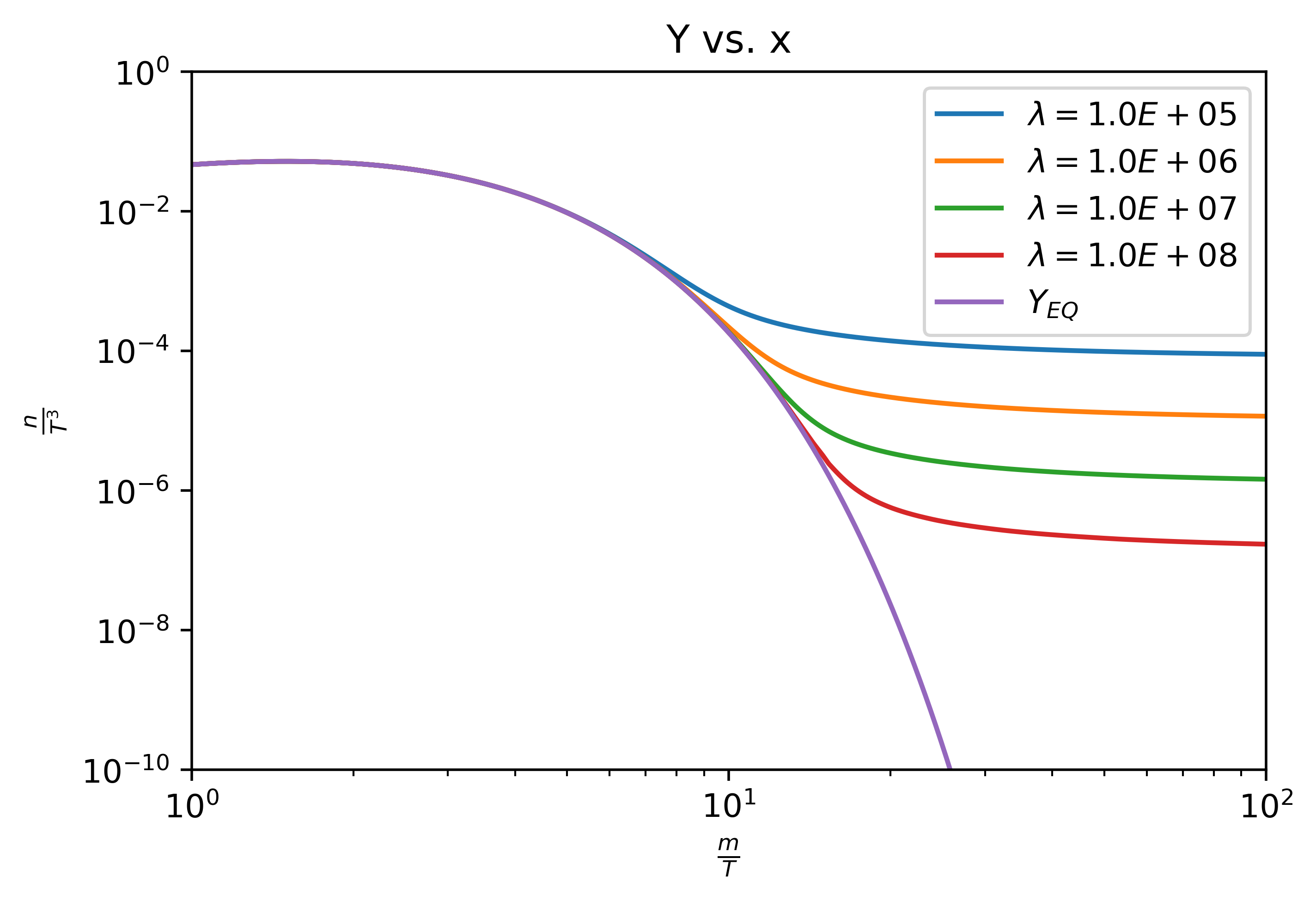
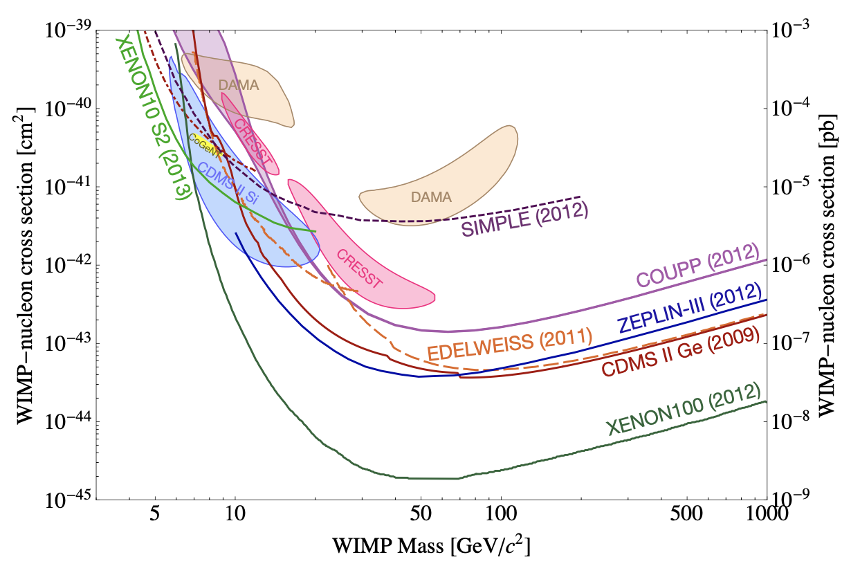
As we can see in the generated plot above, smaller vales of \( \lambda \) cause the relic abundance of WIMP to increase. The time at which reactions cannot occur fast enough to maintain equilibrium is known as the epoch of freeze out, which is denoted as \( x_{f} \). Using the above plot with values of \( \lambda \) (which we assume are generally correct), we can provide an estimate for the epoch of freeze out as \( x_{f} \approx 10 \) based on where the individual curves depart from the equilibrium curve. We can see that at late times \( Y>>Y_{EQ} \), and thus taking 3.52 we can write: $$ \frac{dY}{dx} \simeq -\frac{\lambda Y^{2}}{x^{2}} \tag{3.54}$$ With the assumption that \( Y_{f} \) (\( Y \) at freeze-out) is much larger than \( Y_{\infty} \), we can take the integral of both sides of 3.54 from \( x_{f} \to \infty \) to approximate the relic abundance over temperature cubed as: $$ Y_{\infty} \simeq \frac{x_{f}}{\lambda} = \frac{10}{\lambda} \tag{3.56}$$ We can use this approximation to aid in calculating the present day density of dark matter. After freeze-out, the dark matter density can be expected to fall off proportional to \( a^{-3} \) (as space expands). This gives the expression: $$ \rho_{X} = mY_{\infty}T_{0}^{3} \left ( \frac{a_{1}T_{1}}{a_{0}T_{0}} \right )^{3} \simeq \frac{mY_{\infty}T_{0}^{3}}{30} $$, where \( a_{1} \) and \( T_{1} \) correspond to a late time and temperature where $Y$ has reached its value \( Y_{\infty} \). Thus, we can substitute our approximation in 3.56 and divide by the critical density to get: $$ \Omega _{X} = \frac{x_{f}}{\lambda} \frac{mT_{0}^{3}}{30 \rho_{crit}} = \frac{H(m)x_{f}T_{0}^{3}}{30m^{2}\left<\sigma v \right> \rho_{crit}} \tag{3.58}$$ Using the equation for energy density in the radiation era, we can replace \( H(m) \) with \( g_{*}(m) \) as a function of temperature: $$ \Omega _{X} = \left [ \frac{4 \pi ^{3} G g_{*}(m)}{45} \right ]^{\frac{1}{2}} \frac{x_{f}T_{0}^{3}}{30 \left<\sigma v \right> \rho_{crit}} \tag{3.59}$$ The temperature at dark matter production \( T_{0} \) is roughly \( 100 \text{ GeV} \), \( x_{f} \) is roughly \( 10 \), and \( g_{*} \) is on the order of \( 100 \). Normalizing \( g_{*} \) and \(x_{f} \) and using the estimation of dark matter density \( \Omega_{dm} \simeq 0.3 \) we can write: $$ \Omega _{X} = 0.3 h^{-2} \frac{x_{f}}{10} \frac{g_{*}(m)}{100} \frac{10^{-39}cm^{2}}{\left<\sigma v \right>} \tag{3.60} $$ Thus, our estimate for the cross section of WIMP is on the order of \( 10^{-39} \text{ cm}^{2} \), which agrees with several theories such as supersymmetry. Cushman et. al. provide the figure below that displays WIMP mass and cross section estimates from various studies. We can see that our estimate for WIMP cross section is within reason.

Temperature Dependence of Thermally Averaged Cross Section
The original plot of \( Y \) as a function of \( x \) for various \( \lambda \) relied on the fact that the average temperature cross section \( \left<\sigma v \right> \) is temperature independent. There are many theories in which the cross section does in fact depend on temperature. We can model this as: $$ \left<\sigma v \right> = \begin{cases} A T^{n}=A(\frac{m_{X}}{x})^{n}=Am_{X}^{n}x^{-n} & \text{ for } n=-2,-1,0,1,2 \end{cases}$$ For some constant value \( A \). This temperature dependence alters our equation 3.51. Thus, \( \frac{dY}{dx} \) becomes: $$ \frac{dY}{dx} = - \frac{\lambda}{x^{2+n}} \left\{Y^{2}-Y_{EQ}^{2} \right\} $$ $$ \lambda_{n} \equiv \frac{Am_{X}^{3+n}}{H(m)} $$ We can visualize how temperature dependency of the thermally averaged cross section \( \left<\sigma v \right> \) affects the relic abundance of dark matter by plotting \( Y \) as a function of \( x \) while only varying \( n \). For the sake of this demonstration, I will keep \( \lambda_{n}=10^{5} \).
Numerical Analysis
# calculate values for Y using odeint for multiple n
nvec = np.linspace(-2,2,5)
xrange = np.logspace(0,2,1000)
for i in range(len(nvec)):
    n = nvec[i]
    l = 10**5
    yvalues = odeint(f,yeq(1),xrange,args=(l,n))
    nval = n
    plt.loglog(xrange,yvalues,label=r'$n={}$'.format(nval))

# calculate values for Yeq using previous function (not dependent on n)
yeqvec = np.zeros((1000,1))
for i in range(len(xrange)):
    xtemp = xrange[i]
    yeqvec[i] = yeq(xtemp)

# plot Yeq
plt.loglog(xrange,yeqvec,label=r'$Y_{EQ}$')

# set plot axes limits and labels
plt.xlim([1,100])
plt.ylim([10**(-10),10**(0)])
plt.xlabel(r"$\frac{m}{T}$")
plt.ylabel(r"$\frac{n}{T^{3}}$")
plt.title(r'Y vs. x')
plt.legend()
plt.show

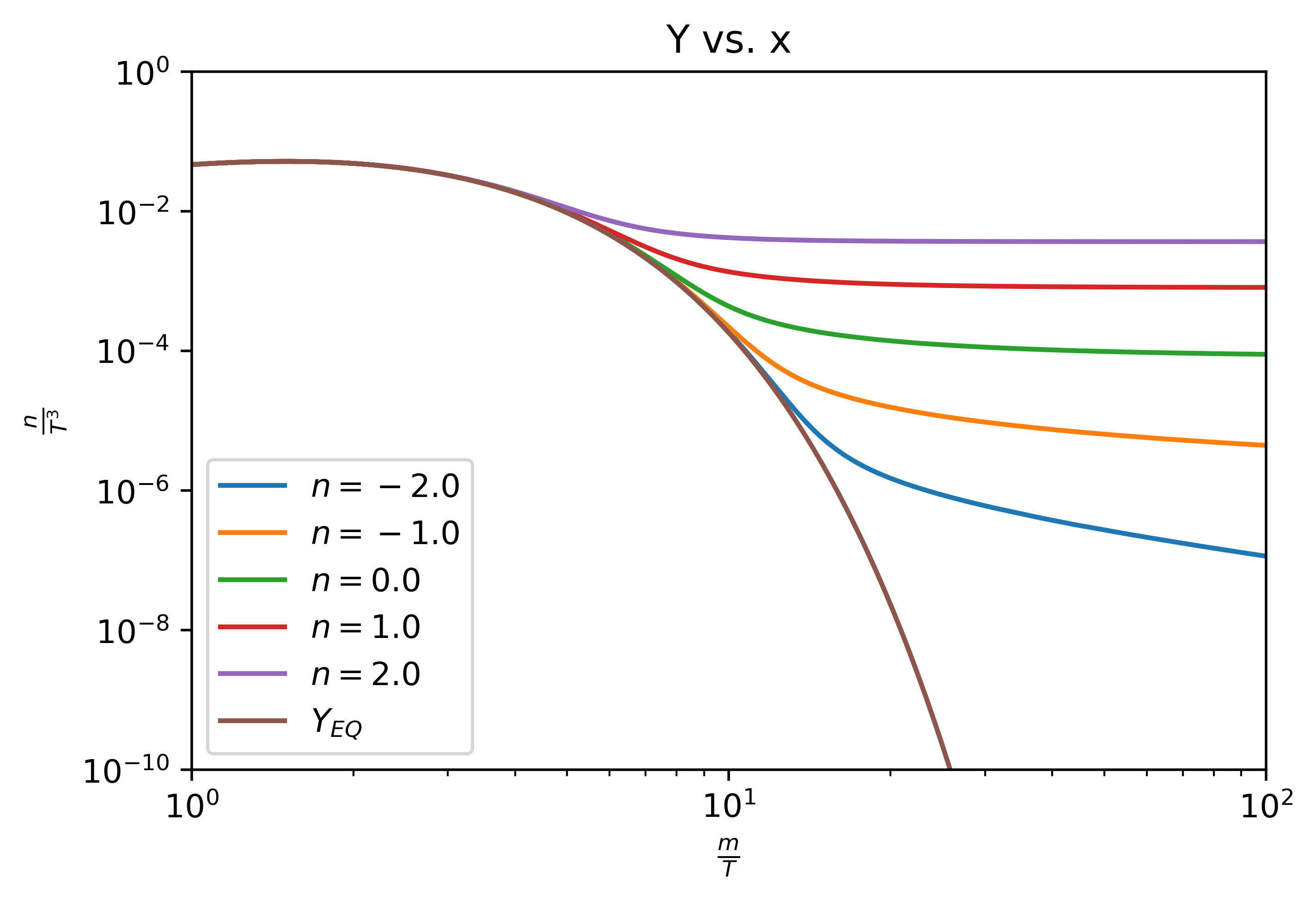
In the above plot we can see that the dark matter relic abundance is affected by a temperature dependent thermally averaged cross-section. For smaller values of \( n \) in our equation, we see that the relic abundance decreases. This makes sense, since for \( n<0 \) the thermally averaged cross section increases in magnitude as \( x \) increases. This increase in cross section is analagous to an increase in \( \lambda \) in the first plot, which had shown a decrease in relic abundance as \( \lambda \) increases.
References
[1] Dodelson, S. (2003). Modern Cosmology. Academic Press An Imprint of Elsevier.